The Basic Architecture of Neural Networks
In this post, we will see the single-layer and multi-layer neural networks. In the single-layer network, a set of inputs is directly mapped to an output by using
a generalized variation of a linear function. This simple instantiation of a neural network is also referred to as the perceptron.
In multi-layer neural networks, the neurons are arranged in layered fashion, in which the input and output layers are separated by a group of hidden layers.
This layer-wise architecture of the neural network is also referred to as a feed-forward network.
This post will discuss both single-layer and multi-layer networks.
Single Computational Layer: The Perceptron
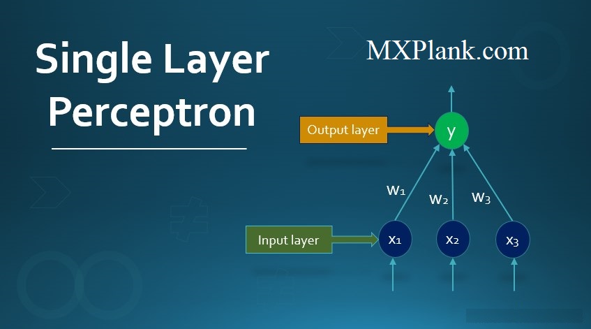
The simplest neural network is referred to as the perceptron. This neural network containsa single input layer and an output node.
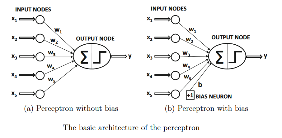
The basic architecture of the perceptron is shown in the above image.
Consider a situation where each training instance is of the form (X̄,y),where eachX=[x
1,...x
d]contains d feature variables,
and y∈{-1,+1} contains the observed valueof the binary class variable.
By "observed value" we refer to the fact that itis given to us as a part of the training data,
and our goal is to predict the class variable forcases in which it is not observed.
For example, in a credit-card fraud detection application,
the features might represent various properties of a set of credit card transactions (e.g.,amount and frequency of transactions),
and the class variable might represent whether ornot this set of transactions is fraudulent.
Clearly, in this type of application, one would havehistorical cases in which the class variable is observed,
and other (current) cases in whichthe class variable has not yet been observed but needs to be predicted.
The input layer contains d nodes that transmit thed features X=[x
1...x
d] with edges of weight W=[w
1...w
d] to an output node.
The input layer does not performany computation in its own right.
The linear function
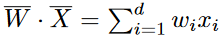
is computed atthe output node.
Subsequently, the sign of this real value is used in order to predict the dependent variable of X.
Therefore, the prediction ŷ is computed as follows:
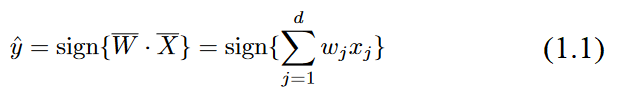
The sign function maps a real value to either +1 or-1, which is appropriate for binaryclassification.
Note the circumflex on top of the variableyto indicate that it is a predicted value rather than an observed value.
The error of the prediction is therefore E(X̄)=
y-ŷ which is one of the values drawn from the set{-2,0,+2}.
In cases where the error value E(X̄) is nonzero, the weights in the neural network need to be updated in the (negative)direction of the error gradient. As we will see later, this process is similar to that used invarious types of linear models in machine learning.
In spite of the similarity of the perceptron with respect to traditional machine learning models,
its interpretation as a computationalunit is very useful because it allows us
to put together multiple units in order to create far more powerful models than are available in traditional machine learning.
The architecture of the perceptron is shown in the above image, in which a single input layer transmits the features to the output node.
The edges from the input to the output containthe weights w
1...w
d with which the features are multiplied and
added at the output node.Subsequently, the sign function is applied in order to convert the aggregated value into aclass label.
The sign function serves the role of anactivation function. Different choicesof activation functions can be used to simulate
different types of models used in machinelearning, like least-squares regression with numeric targets,thesupport vector machine,
or alogistic regression classifier.
Most of the basic machine learning models can be easilyrepresented as simple neural network architectures.
It is a useful exercise to model traditionalmachine learning techniques as neural architectures,
because it provides a clearer picture ofhow deep learning generalizes traditional machine learning.
This point of view is explored later in the coming posts. It is noteworthy that the perceptron contains two layers,
although the input layer does not perform any computation and only transmits the feature values.
The input layer is not included in the count of the number of layers in a neural network.
Since the perceptron contains a singlecomputationallayer, it is considered a single-layernetwork.
In many settings, there is an invariant part of the prediction, which is referred to asthebias.
For example, consider a setting in which the feature variables are mean centered,but the mean of the binary class prediction
from {-1,+1}is not 0. This will tend to occur in situations in which the binary class distribution is highly imbalanced.
In such a case,the aforementioned approach is not sufficient for prediction.
We need to incorporate anadditional bias variablebthat captures this invariant part of the prediction:
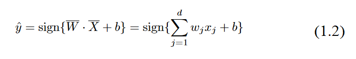
The bias can be incorporated as the weight of an edge by using abias neuron.This is achieved by adding a neuron that always transmits a value of 1 to the output node. Theweight of the edge connecting the bias neuron to the output node provides the bias variable.An example of a bias neuron is shown in Figure1.3(b). Another approach that works wellwith single-layer architectures is to use afeature engineering trickin which an additionalfeature is created with a constant value of 1. The coefficient of this feature provides the bias,andonecanthenworkwithEquation1.1. Throughout this book, biases will not be explicitlyused (for simplicity in architectural representations) because they can be incorporated withbias neurons. The details of the training algorithms remain the same by simply treating thebias neurons like any other neuron with a fixed activation value of 1.
Therefore, the following will work with the predictive assumption of Equation1.1, which does not explicitly usesbiases.
At the time that the perceptron algorithm was proposed by Rosenblatt , these op-timizations were performed in a heuristic way with actual hardware circuits, and it was notpresented in terms of a formal notion of optimization in machine learning (as is commontoday). However, the goal was always to minimize the error in prediction, even if a for-mal optimization formulation was not presented. The perceptron algorithm was, therefore,heuristically designed to minimize the number of misclassifications, and convergence proofswere available that provided correctness guarantees of the learning algorithm in simplifiedsettings. Therefore, we can still write the (heuristically motivated) goal of the perceptronalgorithm in least-squares form with respect to all training instances in a data set
D containing feature-label pairs:
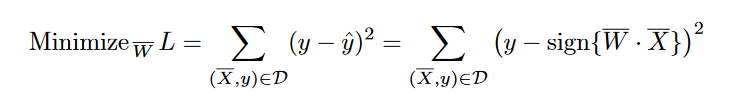
This type of minimization objective function is also referred to as a loss function. As we will see later, almost all neural network learning algorithms are formulated with the useof a loss function. this loss function looks a lot like least-squares regression. However, the latter is defined for continuous-valued target variables,and the corresponding loss is a smooth and continuous function of the variables. On theother hand, for the least-squares form of the objective function, the sign function is non-differentiable, with step-like jumps at specific points. Furthermore, the sign function takeson constant values over large portions of the domain, and therefore the exact gradient takeson zero values at differentiable points. This results in a staircase-like loss surface, whichis not suitable for gradient-descent. The perceptron algorithm (implicitly) uses a smoothapproximation of the gradient of this objective function with respect to each example
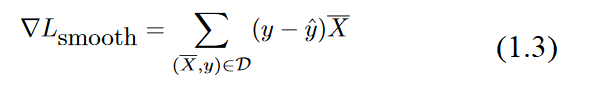
Note that the above gradient is not a true gradient of the staircase-like surface of the (heuristic) objective function, which does not provide useful gradients. Therefore, the staircase issmoothed out into a sloping surface defined by the perceptron criterion. The properties of the perceptron criterion will be described in later posts. It is noteworthy that concepts likethe "perceptron criterion" were proposed later than the original paper by Rosenblatt in order to explain the heuristic gradient-descent steps. For now, we will assume that theperceptron algorithm optimizes some unknown smooth function with the use of gradientdescent.
Although the above objective function is defined over the entire training data, the training algorithm of neural networks works by
feeding each input data instance X̄ into the network one by one (or in small batches) to create the prediction ŷ.
The weights are then updated, based on the error value E(X̄)=(y-ŷ).
Specifically, when the data point X is fed into the network, the weight vector W̄ is updated as follows:
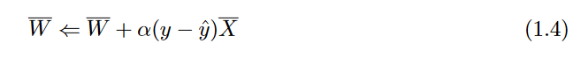
The parameter a regulates the learning rate of the neural network. The perceptron algorithm repeatedly cycles through all the training examples in random order and iteratively adjuststhe weights until convergence is reached. A single training data point may be cycled throughmany times. Each such cycle is referred to as anepoch. One can also write the gradient-descent update in terms of the error
E(X̄)=(y-ŷ) as follows:
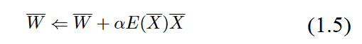
The basic perceptron algorithm can be considered a stochastic gradient-descent method,which implicitly minimizes the squared error of prediction by performing gradient-descentupdates with respect to randomly chosen training points. The assumption is that the neuralnetwork cycles through the points in random order during training and changes the weightswith the goal of reducing the prediction error on that point. It is easy to see from the above Equation that non-zero updates are made to the weights only when
y!=ŷ,
which occurs only when errors are made in prediction. In mini-batch stochastic gradient descent, the aforementioned updates of the equation in the above image are implemented over a randomly chosen subset of
training points S:
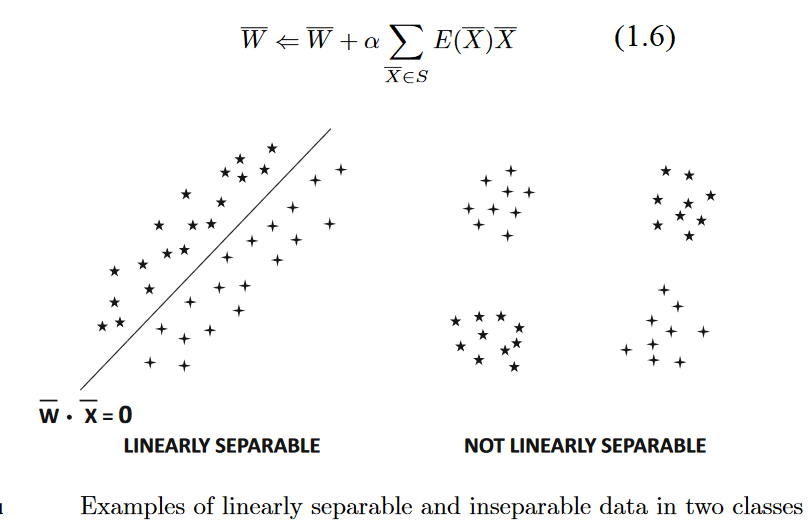
The advantages of using mini-batch stochastic gradient descent are discussed later. An interesting quirk of the perceptron is that it is possible to set the learningrateato 1, because the learning rate only scales the weights.The type of model proposed in the perceptron is alinear model, in which the equation
W̄.X̄= 0 defines a linear hyperplane. Here,W=(w
1...w
d)is a d-dimensional vector that is normal to the hyperplane. Furthermore, the value of W̄.X̄ is positive for values of X̄ on one side of the hyperplane, and it is negative for values of X on the other side. This type ofmodel performs particularly well when the data islinearly separable. Examples of linearly separable and inseparable data are shown in the above image.The perceptron algorithm is good at classifying data sets like the one shown on theleft-hand side of the image above, when the data is linearly separable. On the other hand, it tendsto perform poorly on data sets like the one shown on the right-hand side of the above image.
This example shows the inherent modeling limitation of a perceptron, which necessitates the useof more complex neural architectures.Since the original perceptron algorithm was proposed as a heuristic minimization ofclassification errors, it was particularly important to show that the algorithm convergesto reasonable solutions in some special cases. In this context, it was shown that theperceptron algorithm always converges to provide zero error on the training data whenthe data are linearly separable. However, the perceptron algorithm is not guaranteed toconverge instances where the data are not linearly separable. For reasons discussed inthe next section, the perceptron might sometimes arrive at a very poor solution with datathat are not linearly separable (in comparison with many other learning algorithms)